![]()
This project is a collection of simulations and animations in a couple of domains–namely, celestial mechanics, chemistry, and just plain fun. Most of them sprang out out of a desire to gain a more practical understanding of how physical systems can be simulated in silico, which I felt would better ground my research in computational chemistry. Though the systems presented here are incredibly simple compared to any of the ones I research, I think the exercises contained here were fruitful and very fun.
Acknowledgements
The gases simulations are derived from code written by Jake Vanderplas
(email: vanderplas@astro.washington.edu). Specifically, the balls_in_box.py file
contains the original ParticleBox class (modified only to remove gravity) from
Jake’s animation tutorial
as well as the same basic animation code for the box itself. Calculation of the speed distribution
and animation of the histogram was added. Jake’s original BSD License statement has
been left at the top of the balls_in_box.py file.
I owe the idea for plotting the the M-B distribution as a histogram under the ParticleBox simulation to this gif on Wikipedia created by user Dswartz4 and licensed under the Creative Commons BY-SA 4.0 license. Why did I want to repeat what was already available? I took the goal of re-creating the figure as a useful exercise, and I also wanted to have code that I could then re-use for similar problems.
Installation
I would recommend setting up a virtual environment for running these scripts and notebooks. I have tested this code using python 3.7, but it will probably work with 3.5 or newer. The dependencies are minimal–Numpy, Matplotlib, Jupyter (if you want to run any of the notebooks), and ffmpeg (to save your animations). Here are two options for getting this all installed.
1. Using virtualenv and pip I have frozen my working environment in full_env.txt, so the environment can be recreated with
pip install -r full_env.txt
in your virtualenv to get the necessary dependencies. The weird name for the requirements is to avoid conflicts with building the environment on Binder when sharing notebooks. In order to display animations in the notebook, however, you will also need to make sure that ffmpeg is installed on your machine.
2. Using conda
Alternatively, environment.yml can be used to create a conda environment that includes
ffmpeg. This is the environment used for sharing the contained notebooks on Binder.
If you are a conda user, then, just run
conda env create -f environment.yml
Binder
If you want to run the notebooks in this repository but don’t want to install anything on your own computer, you can explore the repository on Binder. Binder builds a Docker container containing a conda environment with all of the project dependencies and allows you to run and change any of the notebooks in the repo interactively in your browser!
Currently, only the gas simulations are included as a notebook and available on Binder. In the future, it may be possible to make all of the code available in this way.
Organization
The repository groups the simulations roughly by topic into sub-directories of the dynamics directory. Each topic sub-directory contains all of the code needed for the sims but videos of the sims are then grouped together in the videos directory within the project root to make them easier to find.
Gravity
These simulations involve integration on Newton’s equations of motion within an inverse r potential between bodies.
-
projectile.py: Classic projectile motion from your high school physics course, but with the curvature of the ground accounted for. Drag is ignored. This was inspired by my love of the javelin, as can be inferred by the shape of the projectile. When I get some free time, I would love to add in drag and the pitch moment of the javelin–for another time I suppose.- 2-D planar projectile motion for point mass
- include surface curvature
- change gravity and surface curvature (how far would it fly on the moon!?)
- drag
- more complex projectile geometries
To play around with the sim, tweak the last few lines of the script.
if __name__ == "__main__":
    h0 = 2                   # the initial height above the ground (m)
    v0 = np.array([26, 15])  # initial velocity as vx, vy

    # rg is the radius (m) of the surface the projectile is launched from - Earth's radius here
    # g - m/s - 9.8 for Earth
    # dt, nmax - time step (s), maximum number of time steps
    jav = Projectile(h0, v0, rg=6.731e6, g=9.8, dt=0.05, nmax=30000)
Then just run it from your terminal with
python projectile.pyYou should get a pop-up video that looks something like this!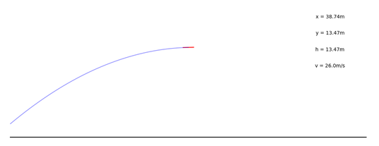
-
many_planet.py: A many body problem where planets are initialized with positions, velocities, and weights, and the system is allowed to evolve. The units are really dummy units, and in the inverse r potential, G is set to 1, giving the force acting on body i by body j as
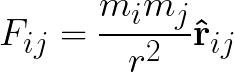
The G term is included at the top of the file, though, and you are welcome to change it and all of the masses and times you would like to simulate to your choice of units. The mechanics should be the same, and I found it simpler to just focus on the relative sizes of the bodies.
- 2-D multi-body interactions
- inverse r potential
- arbitrary initial conditions
To set up a simulation, alter the contents of the Initial State block of code
Below, we define 6 bodies in the array initial. Each row in the array is a body,
and the columns are rx, ry, vx, vy. We specify the mass of each body in the ms
array in arbitrary units, and control the look of the bodies in our plot with the
sizes (marker size) and colors lists
  # Initial State
  initial = np.array([[0, 0, 0, 0],
                      [7, 0, 0, 25],
                      [10, 0, 0, 15],
                      [15, 0, 0, 17.5],
                      [25, 0, 0, 14],
                      [35, 0, 0, 11]])
  ms = np.array([5000, 0.2, 0.1, 1, 0.4, 0.1])
  sizes = [30, 5, 3, 12, 10, 3]
  colors = ['r', 'k', 'b', 'g', 'y', 'm']
This particular setup should yield something like
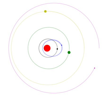
But we can easily tweak the starting conditions to end up with some pretty cool phenomena, like these two massive bodies “orbiting each other”
You may need to change the plot axes and time step to make your simulation run and animate smoothly. Look for the following lines to change
  # Plotting Stuff
  dt = 1 / 120    # simulation timestep

  # Plot Stuff
  # set up figure and animation
  fig = plt.figure(figsize=(10,10))
  ax1 = fig.add_subplot(111, aspect='equal', autoscale_on=False,
                        xlim=(-40, 40), ylim=(-40, 40))
The animations do seem to slow a bit with time, but this doesn’t seem to be too big of an issue for just a few bodies!
-
gravity_1body.ipynb: This is a very short notebook for playing around with the simplest 1 body case and makes it easier to get familiar with the code. You can play around with initial conditions for a single “planet” orbiting the “sun”, and the plot will display the orbit, colored according to the time elapsed.
Gases
These simulations came about while I was teaching tutorials for first-year chemistry at the University of Victoria about ideal gases and the Kinetic Molecular Theory of Gases. As mentioned above, the ideas for these simulations are nothing new, and I borrowed code for the ParticleBox class.
Everything is contained in Gas_Sims.ipynb. You can explore it by running
jupyter notebook
and then clicking on the notebook in the navigator that appears in your browser, so long as you have your environment configured as described above. Alternatively, the notebook can be run on Binder.
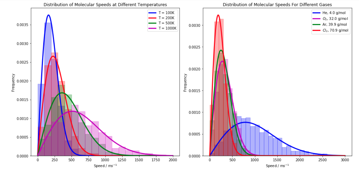
This notebook covers Kinetic Molecular Theory of Gases. It includes plots of the Maxwell-Boltzmann distribution for different temperatures and particle masses:
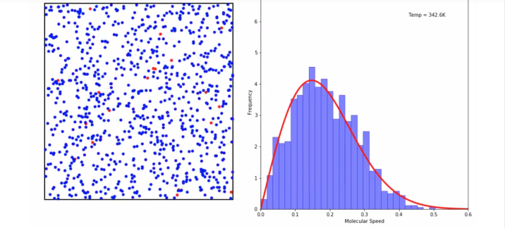
In addition, it has a simulation of particles in a 2D box with the associated speed distribution
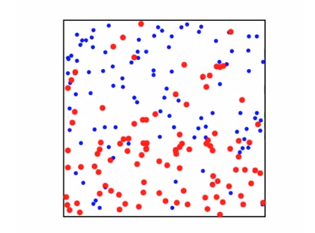
and a diffusion simulation for gases with different masses
Random
Here I have a silly animation that isn’t really a simulation at all. It does, however, involve some time evolution of traveling and stationary waves, so I have included it here. I call him Animan!!!
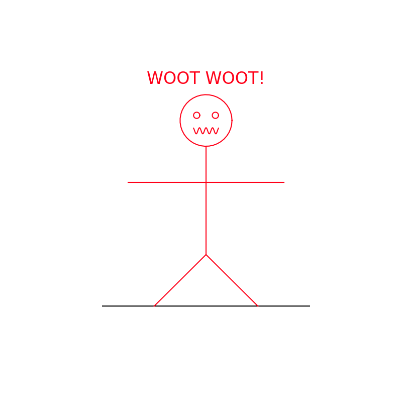
To run animan for yourself, just run
python animan.py
in your terminal. Have fun making him do new dances by tweaking the code, too!