Maximum Cut on a D-Wave QPU

Introduction

This summer (2020), I have been attending a series of online lectures and tutorials entitled Cornerstone Models of Quantum Computing being put on by Quantum BC, TRIUMF and the Helmholtz Institute. The goal is to familiarize students from a range of disciplines with the basic theory and physical implementation of the key ways that quantum computing has been conceived and put into practice thus far, including gate-based models, quantum annealing, measurement-based models, and continuous variable quantum computing. Each week, we apply the theory to exercises that we complete within the computing framework of one of the industry partners of the program. This week, we have been learning about quantum annealing and completing exercises using D-Wave Systems' Leap IDE and Ocean software development kit.

As an introduction to the types of problems that can be embedded on a quantum processing unit (QPU) and solved with a quantum annealing approach, we were asked to solve the Maximum Cut problem. In this post, I would like to share my solution to the exercise. I'm sure there have been many posts written about solving the Max Cut problem before, and in fact D-Wave has a solution posted in their examples. I still thought it would be fun to go through my problem solving process and attempt to explain it. I'm sure that I am not alone in learning most when I am forced to explain myself! At any rate, I hope this can be informative and perhaps help you get started running your own jobs on a QPU!

What is Quantum Annealing?

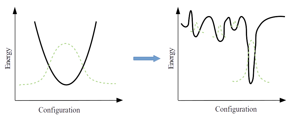
In order to solve the max cut problem on a real quantum computer, we take advantage of a process called quantum annealing. Quantum annealing is a model of computing in which we encode our problem as a set of qubits and the connections, or coupling, between them. We begin with all qubits in a ground state, the lowest energy configuration of states. Then, we slowly change the energy landscape the qubits experience by applying biases to them and their couplings. These biases reflect the problem we want to solve, and we construct them in such a way that the lowest energy state by the end of the annealing, when all biases are applied fully, will be the solution to our problem. Here we are aided by the adiabatic theorem, which basically states that if we have separation between the ground state and the next lowest energy level of our system, and if we change the system (i.e. apply biases) slowly enough, then the system will remain in its ground state throughout the change. Since this ground state represents our problem solution, we can read out the solution by taking measurements, or sampling, the final state of our qubits after applying our biases.

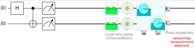
It is worth noting that this computing model differs sharply from gate-based quantum computing, wherein the quantum state of our system is evolved by applying a series of unitary operators, or "gates" to our qubits to obtain a desired state. This gate model is often more familiar to computer scientists and engineers, since it is analogous to the classical gates, such as AND, OR, and XOR gates, which are the foundation of classical computing.

The Maximum Cut Problem

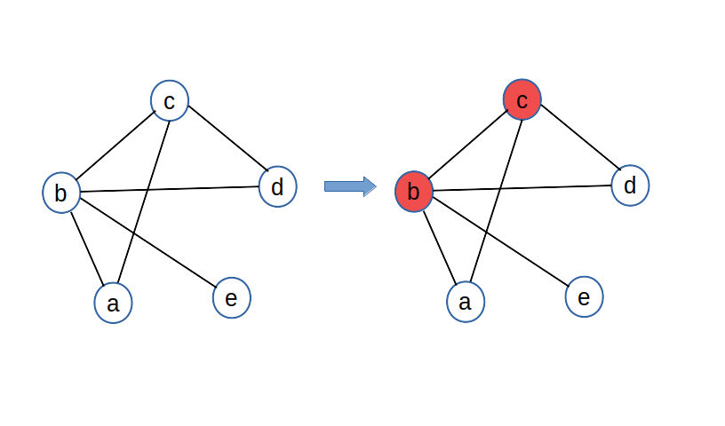
The Max-Cut problem asks us to take a graph and divide its vertices into two subsets such that the number of edges between the two sets is maximized. Since this definition is touch cold and abstract, let's try to understand the problem better with a simple example. In the following graph (left), we have 5 nodes and 6 total edges. We can do some trial and error, perhaps looking to try to intuitively separate the most connected nodes into different groups, and what we come up with is an optimal solution as shown on the right. In this configuration, we make a total of 5 cuts between the white and red groups. We also note that there are actually two best solutions, one with this color set, and the other with the colors simply reversed. In fact, our solutions will always come in pairs.

Problem Solving Strategy

We could solve the Max-Cut problem in a number of ways, including the Ising model, but here we use a Quadratic Unconstrained Binary Optimization (QUBO) formulation. Based on its name, we can infer a some characteristics of QUBO:

1. Quadratic: All terms in QUBO are second order or lower. This means we can only deal with coupling and interaction terms between at most 2 qubits at a time.
2. Unconstrained: Our final formulation will not contain constraints explicitly. This does not mean that our initial problem need have no constraints on the possible values of its variables. Instead, it means that if these constraints exist, they will be combined with our objective function that we want to optimize via a Lagrange multiplier, in effect transforming the constrained optimization into an unconstrained one.
3. Binary: This just means that our variables take on the values 0, or 1, which for qubits would be the two computational basis states.
4. Optimizaton: We want to minimize or maximize some objective function, which will be a measure of how good our solution is. For quantum annealing, we will always be minimizing this function.

To put all of these words a bit more concretely, we can express the energy of a QUBO in mathematical form \[E_{qubo} = \sum_i a_ix_i + \sum_{i,j} b_{ij}x_ix_j\] where \(x_i\) are the binary qubo variables, \(a_i\) are the linear biases that are applied on individual qubits, and \(b_{ij}\) are the quadratic biases applied to coupled qubits. The question now becomes: "How do we express the energy of an undirected graph such that it conforms to this pattern and such that the lowest energy solution will be our Max-Cut partition?"

Luckily for me, during the Cornerstone Models of Quantum Computing lectures, D-Wave provided a set of steps that offer a good process for formulating the problem. I really like this systematic approach and will walk through these steps one by one.

Step 1: Writing the Objective and Constraints

We really have already done this with our problem definition above, but lets now break it up into a statement of objective (the function we would like to minimize) and constraints (which solutions we will accept). Therefore, we can state that our objective is to maximize the number of edges between vertices in different sets. We don't intend to limit in any way how the two sets of vertices can be divided. Therefore, we can say that there are no constraints. Defining the objective and constraints mathematically will come later; for now, we just need to make sure we have a clearly written definition in plain English.

Step 2: Defining Variables

We would like to map our graph vertices to a set of binary variables such that we can "read off" which partition each vertex is in by reading off the value of our variables. Since Max-Cut has us partition the graph into two groups, and since our variables can all take on one of two values, we have a ready mapping. We define a binary variable \(x_i\) for each vertex in the graph. If the variable takes value 0, we say that it belongs to one set, and if it takes value 1, it belongs to the other set. That is \begin{equation*} x_i = \begin{cases} 0 \quad & \text{if} \; i \in \text{set A} \\ 1 \quad & \text{if} \; i \in \text{set B} \\ \end{cases} \end{equation*}

Step 3: Write the Objective Mathematically

We need to write the objective in such a way that edges in the same set increase the energy. If we do this, we can minimize our objective to obtain the solution with the most edges between the two sets. Since we only care about edges here, or the relationships between our variables, let's look at how to write our interaction terms. These are the quadratic terms in the second sum of our \(E_{qubo}\) expression. They define how two qubit pairs interact and therefore model the edges in our graph. Let's write these interaction terms in such a way that when both variables are 0 or both variables are 1 (i.e. both are in the same set), we have an increase in energy, but no increase for variables that are 0 and 1 or 1 and 0. \begin{equation*} E_{qubo} = \sum_{i,j}b_{ij}x_i x_j + \sum_{i,j}b_{ij}(1-x_i) (1-x_j) \end{equation*} Where the sums run over all existing edges between vertices i and j. Notice that terms in the first sum are 1 when both x's are 1, and terms in the second sum are 1 when both x's are 0. All terms are 0 when x's are not equal. Since all edges are equally valued, we can set all of the biases to 1, giving \begin{equation*} E_{qubo} = \sum_{i,j}x_i x_j + \sum_{i,j}(1-x_i) (1-x_j) \end{equation*} Now we can simplify by multiplying out the right hand sum. \begin{equation*} E_{qubo} = \sum_{i,j}x_i x_j + \sum_{i,j}1-x_i-x_j+x_ix_j \end{equation*} Joining the two sums and combining like terms, we have \begin{equation*} E_{qubo} = \sum_{i,j}2x_i x_j-x_i-x_j+1 \end{equation*} It turns out that we can't encode constant energy offsets in the DWave framework. This doesn't matter for our Max-Cut problem, since the constant will only affect the absolute, and not the relative, energies of our solutions. The best solution will remain the best regardless. It does, however, mean that we can simply drop the constant in our expression, giving us the final form of the objective \begin{equation*} E_{qubo} = \sum_{i,j}2x_i x_j-x_i-x_j \end{equation*} Where we remember to only sum over the i, j combinations for edges that actually exist in the graph.

Step 4: Write the Constraints Mathematically

Since we don't have any constraints in this problem, we can skip this step!

Step 5:Combine the Objective and Constraints

Since we only have an objective, we keep the expression that we derived in Step 3. \begin{equation*} E_{qubo} = \sum_{i,j}2x_i x_j-x_i-x_j \end{equation*}

Solve it on the QPU

This is where we will take everything we have derived above and implement it in Ocean, which is D-Wave's software development kit. All of this code was created in D-Wave's Leap IDE. If you would like to follow along with the code, you must create a D-Wave LEAP account. Then you can either start from scratch by creating a new IDE workspace for yourself or simply open my code in the IDE with this link: https://ide.dwavesys.io/#https://github.com/brettrhenderson/MaxCut. You can then run the code directly in this IDE by opening the maxcut.py file and clicking the small green arrow in the top right of the IDE.

Import Packages

from dwave.system import DWaveSampler, EmbeddingComposite
import dwave.inspector as inspector

The first line imports the tools we will need to solve Max-Cut on a D-Wave QPU. DWaveSampler class is the interface that allows us to sample solution states from the D-Wave system. From the distribution of these sampled states after the annealing process, we can identify our lowest energy (optimized) solution. The EmbeddingComposite is a class that handles mapping our defined QUBO to the hardware, the actual qubits in our QPU. It handles the nitty gritty of making sure that the physical coupling between qubits matches the coupling defined in our problem. In some cases, because of the QPU architecture, the embedding composite may not be able to do a one-to-one mapping of variables to qubits and may need to represent a single variable over a chain of qubits. Luckily for us, we can delegate all of this work to the embedding composite for this Max-Cut problem and not think much of it. Lastly, dwave.inspector is a post-processing tool that allows us to see how the problem was embedded in the QPU and visualize our solutions.

Define the Problem

First off, we need a way to represent our graphs. In Max-Cut, we are dealing with un-directed graphs, and we really only care about the connections between vertices. A simple way to capture this is with a set of 2-tuples. Each tuple is an edge containing the names of the two vertices it connects. By this construction, the following code represents the graph that we saw earlier.

graph = {('A', 'B'), ('A', 'C'), ('B', 'C'), ('B', 'D'), ('B', 'E'), ('C', 'D')}

Next, we need to write our objective \(E_{qubo} = \sum_{i,j}2x_i x_j-x_i-x_j\) as a Q matrix, (or dictionary.) From the Ocean documentation, we see that the Q dictionary "Should be a dict of the form {(u, v): bias, …} where u, v are binary-valued variables and bias is their associated coefficient". In fact, we can name our binary variables anything as long as we're consistent. I could just leave them as the names of the vertices in my graph, but I want to make a slight distinction between the variables themselves and what they stand for. Therefore, I settled on prefixing all vertex names with 'x' when converting them to variable names.

What are the coeffiecients, or biases, in our Q matrix? They are the coefficients of each term in the objective function above. Since this is a relatively small problem, we can write out the expanded sum in the objective function to see what is going on. Summing over all edges, in the graph, we get \begin{align*} E_{qubo} = & 2x_A x_B - x_A - x_B + 2x_A x_C - x_A - x_C + 2x_Bx_C - x_B - x_C \\ & + 2x_B x_D - x_B - x_D + 2x_B x_E - x_B - x_E + 2x_C x_D - x_C - x_D \end{align*} And by combining like terms, we can see that all of the cross terms (denoting an edge) have a bias of 2, and all of the linear terms have a coefficient equal to the negative of the number of edges attached to that node. \begin{align*} E_{qubo} = 2x_A x_B & + 2x_A x_C + 2x_Bx_C + 2x_B x_D + 2x_B x_E + 2x_C x_D \\ & - 2x_A - 4x_B - 3x_C - 2x_D - 1x_E \end{align*} As a Q matrix, we write this

graph = {('xA', 'xB'): 2,
     ('xA', 'xC'): 2,
     ('xB', 'xC'): 2,
     ('xB', 'xD'): 2,
     ('xB', 'xE'): 2,
     ('xC', 'xD'): 2,
     ('xA', 'xA'): -2,
     ('xB', 'xB'): -4,
     ('xC', 'xC'): -3,
     ('xD', 'xD'): -2,
     ('xE', 'xE'): -1}

It may seem strange that the negative linear terms from our objective appear in the Q dictionary as quadratic terms (take a look at the last 5 key, value pairs). However, if we remember that in QUBO, \(x_i = x_i^2\), we realize that this quadratic form is actually identical.

Nevertheless, our code would be tedious and somewhat unusable if we had to manually write this Q dictionary for each new graph we wanted to try. Therefore, I have a simple for loop that iterates over the edges in whatever graph we define and generates this dictionary

Q = {}
for edge in graph:
    Q[('x' + edge[0], 'x' + edge[1])] = 2  # edges are unique
    for i in [0, 1]:
        if ('x' + edge[i], 'x' + edge[i]) in Q:  # vertices will come up again and again
            Q[('x' + edge[i], 'x' + edge[i])] -= 1
        else:
            Q[('x' + edge[i], 'x' + edge[i])] = -1

Feel free to step through this code yourself to verify that it does in fact produce the desired Q dictionary for our example, as shown above.

Instantiate a Solver

This code embeds our Q-matrix representation on the physical QPU. We indicate that we would like to use the actual D-Wave sampler, using actual quantum annealing as opposed to simulated annealing, which is also supported in ocean. Then the EmbeddingComposite handles mapping our variables and biases onto the hardware.

solver = EmbeddingComposite(DWaveSampler(solver={'qpu': True}))

Solve the Problem

Next, we run quantum annealing, and take samples from the final distribution of states. Since we have set up our problem such that the lowest energy state is our desired solution, we should see most of our samples landing in this optimized low energy state so long as we take an adequate number of samples, have a decent energy separation between the ground and excited states, and perform annealing slowly enough to obey the adiabatic theory and stay in the ground state.

sampleset = solver.sample_qubo(Q, chain_strength=5, num_reads=50)

If we run this sampling multiple times, we will see that our results are indeed stochastic, with slightly different counts each time. As a result, we may need to play around with the num_reads parameter to ensure that our sample size is large enough to give us a representative picture of the energy landscape and produce all optimal solutions. In addition, we have the ability to tune the value of the chain_strength parameter, which we will discuss more in a moment.

Interpret

Now that we have embedded our problem on the QPU and chosen a sampling methodology, we need a way to read our the solutions that our sampler yields. The easiest way to to this is simply to print the object that is returned when we sample the QUBO.

print(sampleset)

>>>      xA xB xC xD xE energy num_oc. chain_.
0  1  0  0  1  1   -5.0      26     0.0
1  0  1  1  0  0   -5.0      14     0.0
2  1  1  0  1  0   -4.0       2     0.0
3  1  0  1  1  1   -4.0       2     0.0
4  0  1  1  0  1   -4.0       1     0.0
5  0  1  0  1  0   -4.0       1     0.0
6  1  0  0  1  0   -4.0       1     0.0
7  0  0  1  0  1   -4.0       1     0.0
8  1  0  0  0  1   -3.0       1     0.0
9  0  0  1  0  0   -3.0       1     0.0
['BINARY', 10 rows, 50 samples, 5 variables]

This will print out a table of binary strings representing the states of our variables, as shown above. The energy of each state is printed as well, and we can see that our QUBO sampler yielded two lowest energy solutions with energy \(-5.0\). As expected, these two solutions are essentially identical, just with the two sets flipped. That is, in each of them, vertices A, D, and E are in one set, and B and C are in the other. The num_oc. column tells us how many samples were found in each state. In this case, we found 38/50 of the states to represent our optimal solution, with some small population of the next highest energy levels. Finally, the chain_. column shows all 0s, indicating that all of our "chains" are un-broken, a characteristic we will examine shortly when we look back at chain_strength.

inspector.show(sampleset)

This line of code will open up a graphical inspector on the right hand side of the IDE, with a default view containing a "Force-Directed" view of our variables that tries to best show their relationships and biases between them and a solution histogram displaying our results.

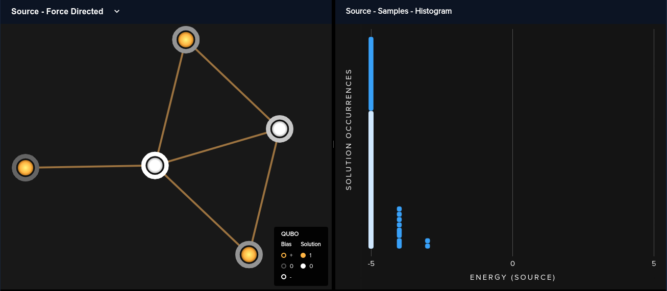
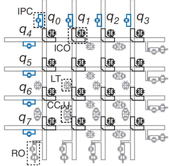
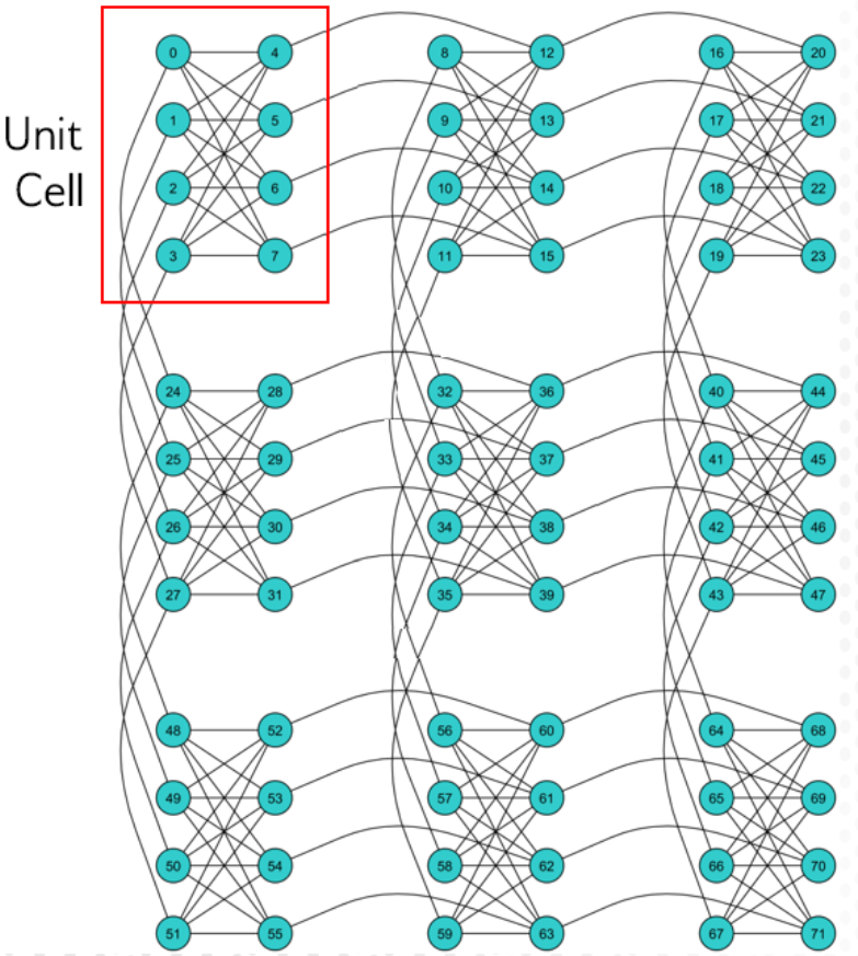
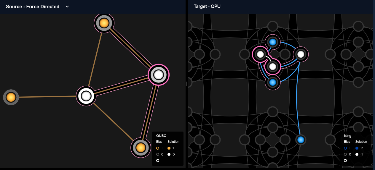
If we click on the small "2" in the upper right corner of the inspector, we get a slightly different view, with the right hand side now showing us how our logical variables have been mapped onto physical qubits. We can hover over a variable on the variables on the left, and the corresponding qubit or qubits will be highlighted on the right. When we hover over variable "xC" in this particular example, we notice something seemingly strange on our QPU. Two qubits are highlighted! In fact, this is not unusual at all. Because physical qubits are only connected in very specific ways in a QPU architecture, sometimes a single qubit cannot be coupled directly to other qubits in the way that our actual variables are coupled. Therefore, the EmbeddingComposite actually splits up a single variable over multiple qubits, called a chain in order to achieve the necessary connectivity. Furthermore, we notice that our graph, despite only having 5 vertices, needed 2 8-qubit unit cells to represent. This, again, is a consequence of the connectivity enabled by the particular architecture of this QPU.

This discussion brings us back to the chain_strength parameter we saw earlier when sampling our QUBO. We have seen that sometimes the embedder must split a single variable over a multi-qubit chain to properly represent the coupling between variables. If this is the case, our hope would be that at the end of our annealing, all of the qubits in that chain would take on the same value. Ocean allows us to enforce this condition by increasing the chain strength, which essentially biases the QPU to ensure that all qubits in a chain end up in the same state. But what happens if we don't enforce this condition? Let's try setting chain_strength=0 and see what we get.

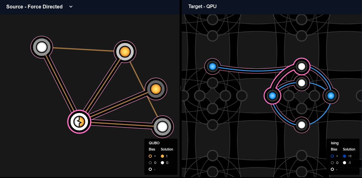
In this run, the embedder has decided to divide variable "xB" into a chain of two qubits. However, these two qubits do not agree in value, giving us a bogus solution. We can also look at our printed solution below and notice that we do not generate the optimal solution with energy \(-5.0\) and we have chain_. values of 0.2, indicating broken chains. The IDE also offers us several warnings of a similar flavor, all of which indicate that we should increase our chain strength. But how much? This can involve some trial and error, but generally we would like the chain strngth to be roughly equal to the magnitude of the largest bias in our QUBO. In our example, we see that the largest bias corresponds to the "most" connected vertex of our graph, "B", and is \(-4.0\). Thus, a chain strength of about 5 should be sufficient.

>>>  xA xB xC xD xE energy num_oc. chain_.
0  1  1  0  1  0   -4.0       5     0.2
1  0  1  1  0  1   -4.0      45     0.2
['BINARY', 2 rows, 50 samples, 5 variables]

Tune the QUBO

Now is our chance to evaluate how well the annealing performed and potentially tune some of our parameters. We should ask ourselves whether we obtained the correct answer. In this case we can probably just go through and validate our solution by hand. In addition, we should check that we have a sufficiently large energy gap between our ground state and the next excited energy levels. In other words, we should examine the energy spectrum of our solutions. Here we see that there is a gap of 1 between our lowest and next lowest energies, which amounts to a 20% difference. In addition, we saw earlier that the vast majority of our QUBO samples were in the lowest energy state. Therefore, we conclude that we don't need to tune our QUBO further.

Conclusions

In this post, I discussed how to derive an objective function that could be minimized to solve the Max-Cut problem on an un-directed graph and walked through an implementation of the solution on a D-Wave quantum annealer using the Ocean SDK. I hope you enjoyed following along and would encourage you to create a D-Wave LEAP account and fiddle around with some code. Try defining a new graph different from our example and explore the solution using the inspector. Do you get the results you expect?!