Island Time - Visualizing Born Effective Charges and Electric Fields in Dielectric Materials

Background

In the study of dielectric and ferroelectric materials, we often need a way to describe the impact of individual atoms or atomic groups on the polarizability of a material. Such a tool might help to explain the role of defects, inclusions, and heteroatoms on their immediate neigborhood and give us a sense of the spatial extent of this effect. Born effective charges are such a tool, in that they tell us the amount that the total polarization of a unit cell of a material changes when we perturb a given atom. A Born effective charge differs from the formal charge on an atom, often significantly. Mathematically, we can define the Born effective charge of an atom \(Z^*\) as a rank 2 tensor, where the element \(Z^*_{ij}\) represents the change in cell polarization in direction \(i\) when the atom is perturbed in direction \(j\). These elements are defined as:

\(Z^*_{ij} = -e\frac{\partial P_i}{\partial r_j}\)

However, these charges can equivalently be defined as the change in the force experienced by the atom when an electric field is applied to the material. That is,

\(Z^*_{ij} = -e\frac{\partial F_i}{\partial E_j}\)

In practice, this derivative is approximated using finite differences, whereby forces are computed under the absence of an electric field and then again with a small applied field \(E\) .

\(Z^*_{ij} = -e\frac{F_{z, field} - F_{z, no field}}{E}\)

This approach is much more efficient for simulations with many atoms since one need only run two single point calculations (one for zero field and one for applied field) to compute a tensor element for all atoms instead of single point calculations where each atom is perturbed in turn.

Pybec is a python package for parsing the output of QuantumEspresso calculations to calculate these Born effective charges. It also contains plotting abilities to visualize born effective charges. This allows a user to see how these charges change in the vicinity of defects and to view interpolated 3-D representations of these charges in the space around such defects, which serves as a proxy for the induced electric field around defect sites when an external field is applied.

Plotting Abilities

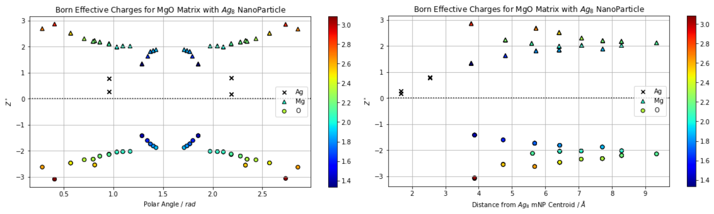
One of the useful abilities of Pybec is that it can plot the radial or angular distribution of Born effective charges relative to some point in your simulation cell. For example, in the following, I have used the CPMD module of QuantumEspresso to optimize a unit cell of MgO with an 8-atom silver inclusion at its center and used Pybec to plot the distribution of the absolute value of the Born effective charges relative to the center of mass of the inclusion.

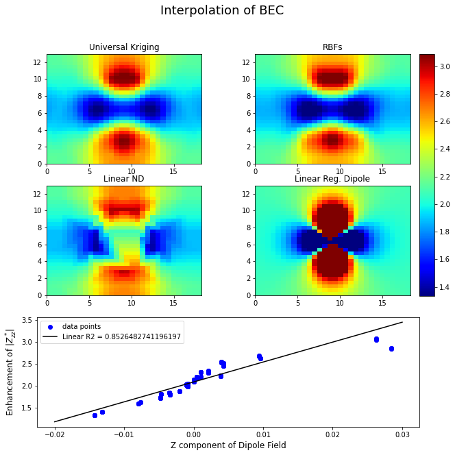
Left: Born effective charges of all atoms plotted
against the polar angle relative to the silver inclusion. Right: Plotted against the distance from the inclusion center. — Left: Born effective charges of all atoms plotted against the polar angle relative to the silver inclusion. Right: Plotted against the distance from the inclusion center.

The notebook included with pybec can also be used to model inclusions as point dipoles and compare the 3D distribution of born effective charges against the field of this dipole at the various atomic coordinates. Below are several methods of 3D interpolation for the calculated Born effective charges shown as a slice through the center of the silver inclusion.

Interpolation of Born
effective charges using Kriging, a radial basis function kernel, and linear interpolation, plus the field of a
point dipole centered at the inclusion center. The bottom plot shows the correlation between the model dipole field and
calculated Born effective charges. — Interpolation of Born effective charges using Kriging, a radial basis function kernel, and linear interpolation, plus the field of a point dipole centered at the inclusion center. The bottom plot shows the correlation between the model dipole field and calculated Born effective charges.

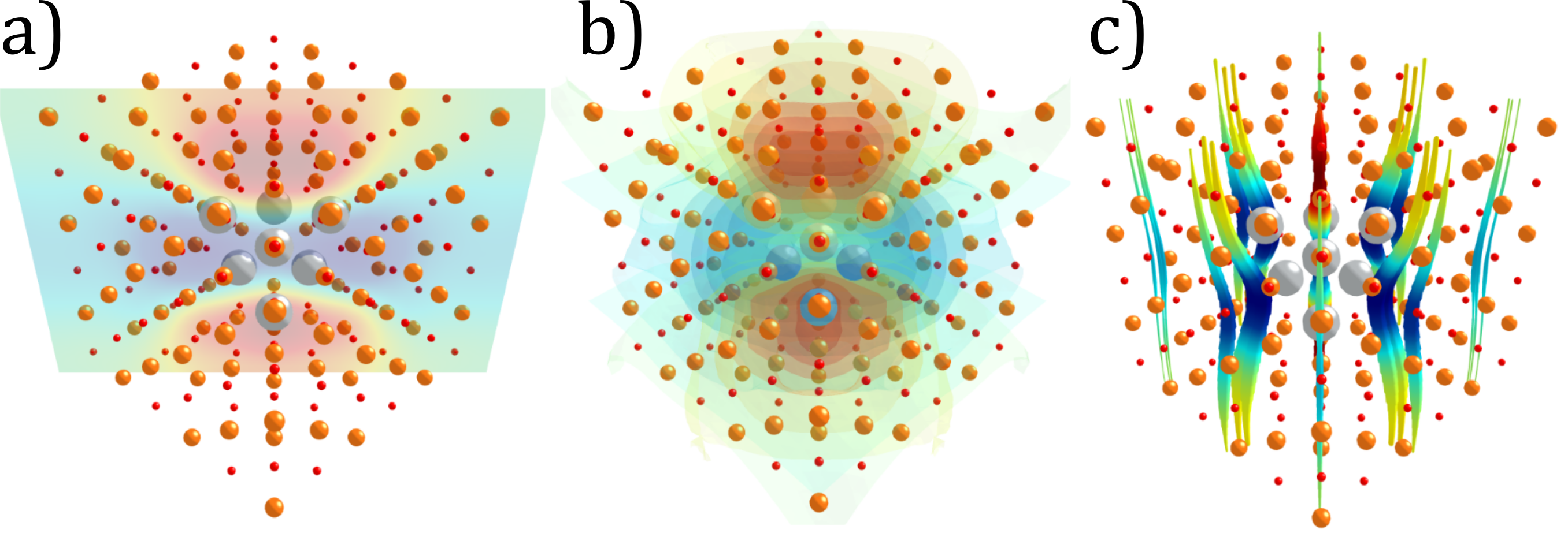
The notebook has its own 3D plotting abilities, enabled by Plotly, which allow one to display the interpolated induced electric field around the inclusion using slices, isosurfaces, and streamlines.

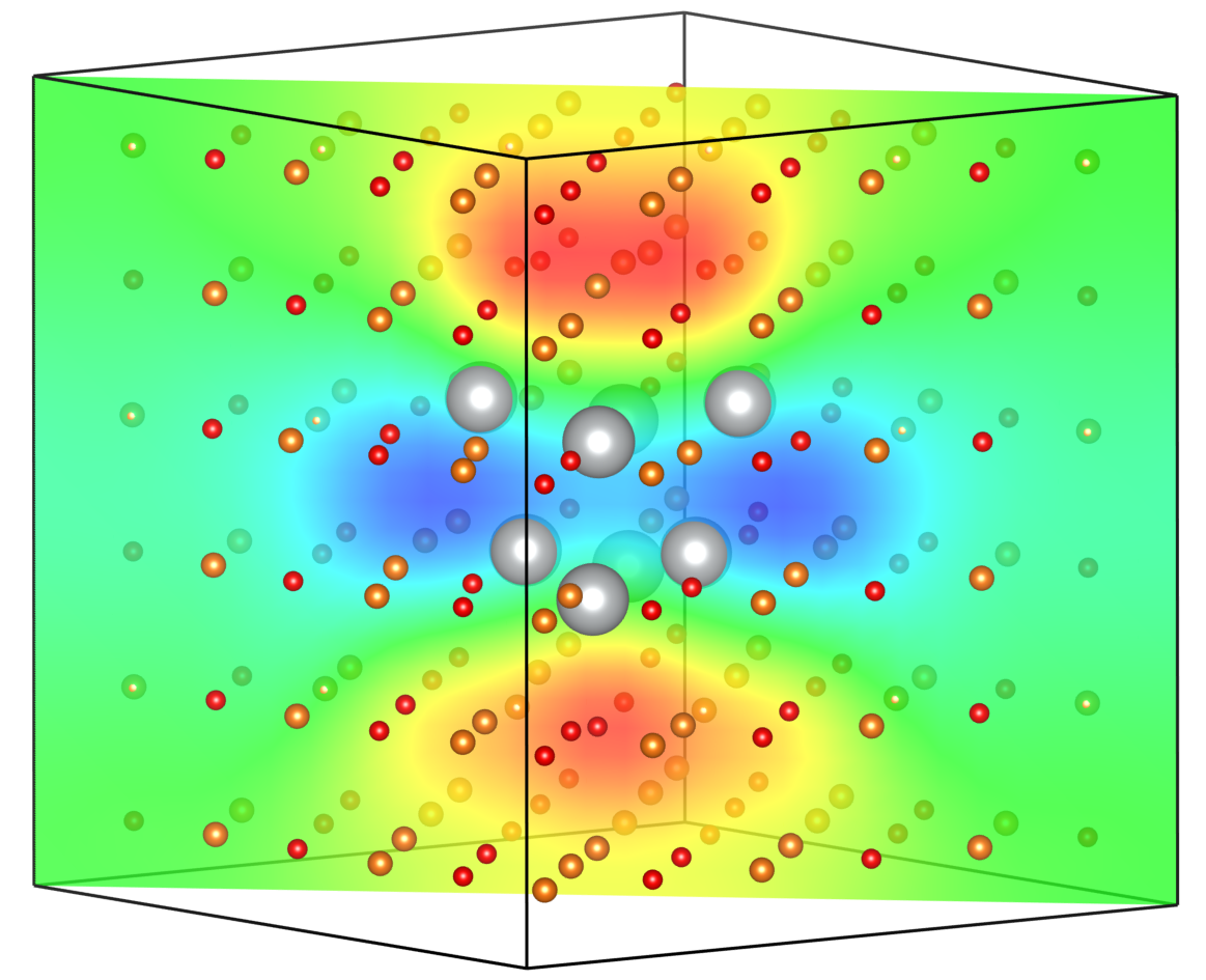
a) Slice of interpolated induced electric field. b) Isosurfaces
of interpolated induced electric field. c) Streamlines of interpolated induced electric field plus external applied field. — a) Slice of interpolated induced electric field. b) Isosurfaces of interpolated induced electric field. c) Streamlines of interpolated induced electric field plus external applied field.

Finally, Pybec can be used to write calculated volumetric data to .XSF files for later plotting and manipulation in your preferred visualization software. For example, here is the interpolated Born effective charge distribution plotted in VESTA.

Interpolated Born effective charges plotted in VESTA.

Installation

The PyBEC Package

PyBEC is available via the Python Package Index (PyPI).

Inside the virtual environment for your project: pip install pybec

Jupyter Notebook

Pybec comes with a jupyter notebook that can walk users through some of its most useful capabilities. To run the notebook, first install PyBEC as discussed above.

Next, download the notebook for a given github release. Download and extract the archive, and run the contained Jupyter Notebook.

Usage

A user manual and API documentation are available online for more detailed instructions on using Pybec.

Copyright

Acknowledgements

Project based on the Computational Molecular Science Python Cookiecutter version 1.3.